
Fan affinity laws are one of the most useful tools in fan engineering. They let you estimate how airflow, pressure, power and noise change when speed, impeller diameter or air density changes — without a new test.
There is one limitation that gets overlooked, and it is expensive.
The well-known cube law describes the change in fan shaft power under similarity conditions. It does not describe the electrical power drawn from the mains. When a fan is slowed down with a variable frequency drive, the aerodynamic load collapses — but the motor is then running at a small fraction of its rated load, and the efficiencies of the motor, the inverter and the mechanical drive all move with it.
This guide works through all three affinity laws with charts, then shows exactly where the cube law stops describing your electricity bill.
What the fan laws say
The fan laws describe how geometrically similar fans behave when speed, size or gas density change. The three variables are rotational speed n, impeller diameter D and density ρ:
Q ∝ n · D³ — volume airflow
Δp ∝ ρ · n² · D² — fan pressure
Pshaft ∝ ρ · n³ · D⁵ — shaft power
Note what is not in the first line: volume airflow does not contain density. A fan is a constant-volume machine at a given speed — it moves the same cubic metres per hour whether the air is cold and heavy or hot and thin. Density appears in pressure and power, not in volume flow.
These relationships come from dimensional analysis, and they hold when model and prototype are geometrically, kinematically and dynamically similar — the three conditions set out in AMCA's derivation of the fan laws (source: AMCA — Derivation of the Fan Laws).
Changing the speed
This is the most common use of the affinity laws, and the reason variable speed control saves so much energy. For the same fan and the same air:
Q₂/Q₁ = n₂/n₁ · Δp₂/Δp₁ = (n₂/n₁)² · P₂/P₁ = (n₂/n₁)³
Drop the speed to 80% and airflow falls to 80%, pressure to 64% and shaft power to 51.2%. A fifth off the speed takes nearly half the shaft power.
The chart below is one 500 mm impeller at five speeds spanning the usual motor range. Logarithmic axes, because a 6:1 speed range is a 36:1 pressure range and a 216:1 power range — on linear axes the 600 rpm curve would be an invisible smudge against the 3600 rpm one.
That dashed parabola is worth dwelling on. It is the locus of the same aerodynamic point at every speed — and it is also the shape of a purely turbulent system curve. That is why a fan on a VFD serving a fixed duct system stays at roughly constant efficiency as it slows: it slides along its own similarity parabola. Add a fixed pressure component, and it does not.
Changing the diameter
At constant speed and density, between geometrically similar fans:
Q ∝ D³ · Δp ∝ D² · Pshaft ∝ D⁵
The fifth power is the one that surprises people. Take 10% off the diameter and airflow falls to 72.9%, pressure to 81% and power to 59%.
These diameter laws assume genuinely similar designs. They scale a 400 mm member of a range to the 630 mm member of the same range. They do not scale one manufacturer's airfoil impeller to another's paddle wheel, and they do not survive a change of blade geometry or casing proportions.
Changing the air density
Density changes with temperature, altitude, humidity and gas composition. At the same speed, the same fan moves the same volume:
Q₂ = Q₁ · Δp₂/Δp₁ = ρ₂/ρ₁ · P₂/P₁ = ρ₂/ρ₁
Take a catalogue curve rated at 1.20 kg/m³ and run the fan on air at 1.00 kg/m³ — roughly 60 °C, or sea-level air at about 1,700 m. The density ratio is 0.833, so at the best-efficiency point of our example fan the airflow stays at 3,477 m³/h, but the pressure falls from 1,291 Pa to 1,076 Pa and the shaft power from 1.56 kW to 1.30 kW.
Two consequences follow, and they pull in opposite directions.
The first is a trap: the fan still delivers its volume, so it looks fine, but it can no longer push through a system that needs 1,291 Pa. Hot-gas and high-altitude selections fail here more often than anywhere else. Our guide to temperature, altitude and fan performance works through the corrections, and the air density calculator gives you the ρ to start from.
The second is a benefit worth remembering: the shaft power falls with density too. A fan selected for hot gas draws less power hot than cold — which is exactly why the motor must be checked at the cold start condition, when the air is dense and the power demand is at its highest.
And because volume stays constant while density drops, mass flow drops with it: ṁ = ρ · Q falls from 1.16 to 0.97 kg/s in the example above. If the process needs kilograms of oxygen rather than cubic metres of air, that is the number that matters.
Reading the laws off a real fan field
Selection software draws the affinity laws as a field rather than a formula: the fan curve at every frequency the drive can produce, with lines of constant shaft power, efficiency or sound laid over it. Two of those overlays show the fan laws directly.
That second chart is the affinity laws in their purest visual form. Slow the fan down along one of those lines and the impeller efficiency does not change at all — 80% at 60 Hz is still 80% at 30 Hz.
Hold on to that fact. It is about to stop being the whole story.
Speed and noise
Fan speed drives acoustics harder than almost anything else. For geometrically similar conditions, sound power scales with the fifth power of speed — 50 log₁₀ in decibel terms:
LW2 = LW1 + 50 · log₁₀(n₂/n₁)
And with diameter at constant speed, 70 log₁₀:
LW2 = LW1 + 70 · log₁₀(D₂/D₁)
Those two coefficients are the same relationship seen from two directions. Sound power follows the fifth power of circumferential speed and separately the square of diameter; since tip speed itself is proportional to diameter at fixed rpm, the diameter exponent comes out as 5 + 2 = 7 (source: Punker — fan acoustics).
Reducing speed by half is worth roughly 15 dB of sound power — an enormous acoustic change, and the single most effective noise measure available on most fan installations.
Speed also moves the spectrum
Slowing a fan does more than lower the overall level: it moves the tonal content. The blade passing frequency is the blade count times the rotational speed (source: Kairouz & Price — Understanding fan acoustics):
fBPF = Z · n / 60
A 6-blade fan at 1,500 rpm puts its blade tone at 150 Hz. Run it at 750 rpm and the tone drops to 75 Hz. Two operating points with similar overall dB(A) can therefore sound completely different, and low-frequency tones are both harder to attenuate and more likely to transmit through structure. Overall levels hide this; octave-band data does not, which is the case our guide to sound power, sound pressure and octave bands makes in detail.
Acoustic scaling is also the least reliable of the fan laws. Measured octave-band data beats a scaled estimate every time; where no measurement exists, the VDI 3731 fan noise calculator gives a screening estimate with its assumptions visible.
The mistake: assuming electrical power follows the cube law
Here is where a clean piece of physics turns into a wrong number on an energy report.
Take a fan needing 10.0 kW at the shaft at full speed. Drop it to 50% speed and the affinity law gives the shaft power immediately:
Pshaft = 10.0 × 0.5³ = 1.25 kW
That is correct. The error is the next step — applying the same factor of 0.125 to the electrical input, and concluding that a system drawing 11.32 kW at full speed now draws 1.41 kW.
It does not. The real system in this example draws 1.71 kW — 21% more.
The reason is that a fan system is a chain, and only its first link obeys the fan laws:
grid → inverter → motor → drive → fan
Each link has losses, and the correct expression is:
Pelectrical = Pshaft / (ηdrive · ηmotor · ηVFD)
None of those three efficiencies is a constant. All three fall as the fan slows — which is exactly when the cube law promises the biggest savings. This is the system decomposition that ANSI/AMCA 207 sets out for fan system input power, and the one we walk through stage by stage in AMCA 207 explained.
A small example that makes the error obvious
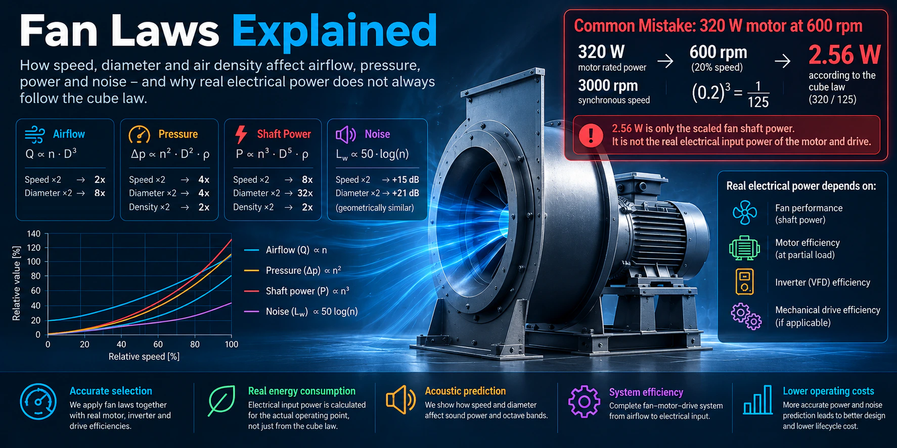
Consider a small industrial centrifugal fan driven by a 320 W motor with a synchronous speed of about 3,000 rpm, run from an inverter at 600 rpm — 20% of speed.
The speed ratio is 0.2, so the cube ratio is 0.2³ = 0.008 = 1/125. Apply that to the motor rating:
320 W / 125 = 2.56 W
A 320 W industrial motor and its inverter do not run a fan on 2.56 W.
Where exactly is the mistake? Two separate things went wrong.
First, the cube law was applied to the wrong quantity. 320 W is the motor's rated power, not the fan's shaft demand at full speed, and certainly not the system's electrical input. The affinity law scales the aerodynamic demand of the fan; it says nothing about a nameplate.
Second, even applied correctly, it only reaches the shaft. The fan here needs about 2.4 W at the shaft at 600 rpm — and the motor and inverter still carry:
- core losses in the iron, which depend on frequency and flux rather than on load,
- the stator current needed to magnetise the machine, which barely falls when the torque does,
- friction and windage,
- inverter switching and control losses, part of which the drive consumes simply by being energised,
- mechanical transmission losses, where a belt or gearbox is fitted.
Those losses are a rounding error at full load. At 0.8% load they are the entire consumption.
The point is emphatically not that variable speed control disappoints. In this example the fan still goes from about 430 W to about 35 W — a 92% saving. The point is narrower and more practical:
The cube law describes the fan. It does not describe the efficiency of the drive system around it.
Motor efficiency at partial load
This is the largest of the three effects, and the one most often ignored.
A motor's nameplate efficiency describes one point: rated load. Motors hold that efficiency well down to about half load, and then give it up. The US Department of Energy puts the turn explicitly below about 40% load, and notes in the same breath that a 20% speed reduction on a fan — which halves the fan power — can drop motor efficiency and power factor to low levels (source: DOE — Improving Fan System Performance; see also Improving Motor and Drive System Performance).
Now put that together with the cube law. Halving the fan speed takes the shaft power to one eighth — so a motor at 93% load goes to roughly 12% load. It has moved from the flat part of that curve deep into the falling part, in one step.
And the motor is sized for the worst case, not the usual one. A fan that spends its life at 60% speed is still fitted with a motor for 100%, which means it spends its life at single-digit load percentages. Using nameplate efficiency at every operating point systematically overstates the savings. How to size it without overdoing it is the subject of choosing the right motor for a fan, and the motor efficiency calculator gives the IEC 60034-30-1 nominal values to start from.
Inverter and drive losses
The inverter is the second link. Modern drives are efficient near their design load — 95–98% is normal — but part of their loss is effectively fixed while they are energised, so efficiency falls at light load just as the motor's does. In our example it goes from 96.9% at full speed to 91.6% at half speed. Some drives reduce motor magnetisation at part load to claw back some of the motor's share, which helps, and is another reason a single fixed efficiency cannot represent the whole range.
The third link is mechanical. A belt drive, gearbox or coupling has its own losses, and they too are partly fixed: our example belt goes from 98.0% to 95.3% between full and half speed. Direct drive avoids this link entirely, which is one of its real advantages.
What this does to overall efficiency
Earlier, the impeller efficiency lines radiated from the origin: the same aerodynamic point gave the same efficiency at every speed. Draw the wire-to-air efficiency on the identical field — air power divided by power drawn from the grid — and the picture changes completely.
Those two charts are the whole argument in one picture. The impeller does not care how fast it turns. Everything between the impeller and the meter does.
It also means the best operating point of a fan and the best operating point of a fan system are not the same point — and only the second one shows up on an electricity bill. The difference between the efficiency definitions is unpacked in fan efficiency explained.
Why a few percent matters
A power prediction error looks small until it is multiplied by a year.
In our worked example the cube law predicted 1.41 kW at half speed and the system draws 1.71 kW — a difference of 0.30 kW. At 6,000 operating hours a year:
0.30 kW × 6,000 h = 1,796 kWh/year
At €0.20/kWh that is about €359 a year, on one fan, from one modelling shortcut. Across a plant with dozens of fans, or over a ten-year life cycle, it stops being a rounding error — and it is the sort of gap that turns a promised payback into a disappointing one.
It matters most in exactly the places where the numbers get quoted hardest: energy audits, life-cycle cost comparisons, FEI and ErP calculations, variable-speed retrofits, fan arrays, data centres and any continuous process. For fan arrays the effect compounds, because staging fans down puts every running motor further down its load curve.
How CloudAir handles this
Our fan selection software does not stop at the cube law. For every operating point it works down the whole chain:
- Fan — airflow, static and total pressure, fan efficiency, shaft power and speed at the actual duty point.
- Mechanical drive — belt or coupling losses where the arrangement has them.
- Motor — efficiency at the actual load, not the nameplate value, which is what makes a part-load prediction honest.
- Inverter — included in the electrical input rather than assumed loss-free.
The result is an electrical input figure, an annual energy figure and a running cost that hold up at 40% speed as well as at 100%. You can see the same chain worked through by hand in the free fan power configurator, and scale a single duty point with the fan laws calculator.
Where the fan laws stop working
The affinity laws are a model, and like any model they have edges:
- Geometry must actually be similar. Different blade forms, casing proportions or tip clearances break the scaling.
- Reynolds number effects. Scaling a small model up, or running a fan very slowly, moves the flow regime and the efficiency with it.
- Compressibility. At high pressure rise, air stops behaving as an incompressible fluid and a compressibility correction is needed.
- Blade angle and control devices. Adjustable-pitch axials and inlet guide vanes change the machine, not just its speed.
- System effect. A bad inlet or a close elbow makes the installed fan behave unlike the tested one, whatever the laws predict (source: AMCA — Mitigating System Effect; see also why a fan does not deliver its expected airflow).
Professional selection should therefore combine measured performance data, the fan laws, the system calculation and the component efficiencies — not any one of them alone.
Fan laws — quick reference
| Change | Airflow | Pressure | Shaft power | Sound power |
|---|---|---|---|---|
Speed n | n | n² | n³ | 50·log(n₂/n₁) |
Diameter D | D³ | D² | D⁵ | 70·log(D₂/D₁) |
Density ρ | unchanged | ρ | ρ | needs its own correction |
| Electrical input | Not given by the fan laws — calculate the drive, motor and inverter at the actual load | |||
Frequently asked questions
Does halving fan speed really cut power to one eighth?
It cuts the fan's shaft power to one eighth, under similarity conditions and with no fixed pressure component in the system. The electrical input falls by less, because the motor, inverter and mechanical drive all become less efficient at the reduced load.
Does air density change the airflow?
No. At a fixed speed the fan moves the same volume regardless of density. Pressure, shaft power and mass flow all change in proportion to density; volume flow does not.
Can I use the fan laws between two different fan models?
Only if they are geometrically similar members of the same range. Between different blade designs, casings or manufacturers the laws do not hold, and the diameter relationships are the first to break.
Why does the error grow as the fan slows down?
Because the fan's demand falls with the cube of speed while a large part of the motor and inverter losses does not fall nearly that fast. The smaller the aerodynamic load, the larger those near-fixed losses are as a share of the total.
Is a VFD still worth it?
Almost always, yes — the savings are large even after the part-load efficiencies are accounted for honestly. In our small example the fan still drops from about 430 W to about 35 W. The correction changes the size of the prize, not its existence.
What should I ask a supplier for?
Electrical input power at each operating point in the duty profile, with the motor efficiency stated at that point's load and the inverter and drive included — not a single nameplate efficiency applied to a cube-law curve.
If you would rather have that calculated for every selection than reconstructed from a catalogue afterwards, that is what our fan selection software does: the fan laws where they apply, and the real efficiency chain where they do not.